 (1)
(1)
While on a brief visit to Fermilab I was asked to look at the strengths of and locations for skew quads in the main injector. In this note we will first set up some notation in which to discuss the coupling and show how the coupling is generated and how it propagates. We will then estimate the amount of coupling produced by two kinds of random errors, roll angles of normal quadrupoles and vertical orbit displacements within sextupoles. Based on these we can make estimates of the strengths of the skew quads required to locally decouple the machine at one point. also based on the way the coupling propagates we can identify good locations for the skew quads. This note presents no new theoretical results; it only applies well known results to the specific case of the main injector.
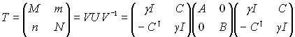
There is a well developed theory of transverse coupling.1,2,3 We will most closely follow the notation of Billing. Let T be the 4 by 4 full turn transfer matrix.
(1)
where A, B, and C are 2 by 2 matricies, I is the 2 by 2 identity matrix and
![]() (2)
(2)
A and B are the full turn transfer matrices for each of the normal modes and so have the form
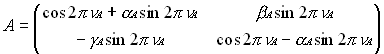 (3)
(3)
and similarly for B. V relates the normal mode coordinates to the horizontal and vertical displacements and angles. Remove the dependence on the Twiss parameters
![]() (4)
(4)
where
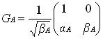 (5)
(5)
![]() can be calculated from
can be calculated from
 (6)
(6)
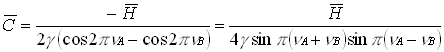
where H = m + n† and ![]() = GAHGB-1
= GAHGB-1
It can be shown that*
(7)
From equation (3), Tr(A - B) = 2(cos2pnA - cos2pnV). Near the coupling resonance, that is at the closet approach of the tunes, Tr2(M - N) = 0, and the two tunes can be written as nA = n+Dnmin/2, and nB = n - Dnmin/2. Putting these into equation (7)
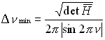 (8)
(8)
![]() can be
written as
can be
written as
(9)
where
 (10)
(10)
Then
![]() (11)
(11)
It can also be shown that the ![]() ± depend of the skew quads as
± depend of the skew quads as
![]() (12)
(12)
where the sum is over all the skew quads, p is the observation point fA,pk is the phase advance of the normal mode A between the kth skew quad and the observation point p, R is a rotation matrix, and q is a normalized skew quad strength
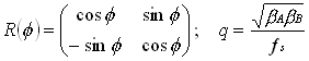 (13)
(13)
where ƒs is the skew focal length and the b's
are evaluated at the location of the skew quad. Notice that equation (12) implies that
there are components of ![]() , and hence
, and hence ![]() ,
that propagate as the sum and as the difference of the normal mode phase advances.
,
that propagate as the sum and as the difference of the normal mode phase advances.
The ![]() ± are the sum
of many terms, one for each couple, each of which is proportional to a rotation matrix.
Each term may be thought of as a vector with a direction given by the angle in the
rotation matrix and an amplitude given by the normalized strenght of the skew quad. The
sum of these terms has the amplitude and direction of the sum of the vectors. If all the
terms are random, the problem is equivalent to a random walk in two dimensions. So the
root mean square (rms) value for the
± are the sum
of many terms, one for each couple, each of which is proportional to a rotation matrix.
Each term may be thought of as a vector with a direction given by the angle in the
rotation matrix and an amplitude given by the normalized strenght of the skew quad. The
sum of these terms has the amplitude and direction of the sum of the vectors. If all the
terms are random, the problem is equivalent to a random walk in two dimensions. So the
root mean square (rms) value for the ![]() ± is
± is
![]() (14)
(14)
where f is a random direction, and N is the number of skew quads. Then
![]() (15)
(15)
Put this into equation (11), and look near the coupling resonance (nA = » nB),
![]() (16)
(16)
And so using equation (8) the closest approach of the tunes will be
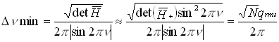 (17)
(17)
This also shows that Dnmin only depends on
![]() +, the
components of
+, the
components of ![]() that propagate as
the difference of the normal mode phase advances. Note that if Dnmin =0 then
that propagate as
the difference of the normal mode phase advances. Note that if Dnmin =0 then ![]() +=0 and since
+=0 and since ![]() + is proportional to a rotation matrix, det
+ is proportional to a rotation matrix, det![]() += 0 implies that
+= 0 implies that ![]() += 0.
+= 0.
A thin quad with inverse focal length Kl that is rolled by an angle q has a skew focal length of 1/ƒs,quad = Kl sin 2q»2Klq, for small q.
A vertical orbit displacement of y in a sextupole of strength Dx'/x2 produces a skew focal length of 1/ƒs,sext=2(Dx'/x2)y.
So the ![]() for the ring will be
for the ring will be
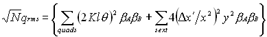 (18)
(18)
At the quads and sextupoles, the factor ![]() does not vary much, so for
this estimate it may be taken out of the sum.
does not vary much, so for
this estimate it may be taken out of the sum.
![]() (19)
(19)
The main injector will have about 208 quads with typical strengths of 0.09/m and about 108 sextupolew with Dx'/s2 of either 0.00485/m2 or -0.00915/m2. Use an rms angle of 1 mrad and a vertical orbit error with rms of 3 mm. Then,
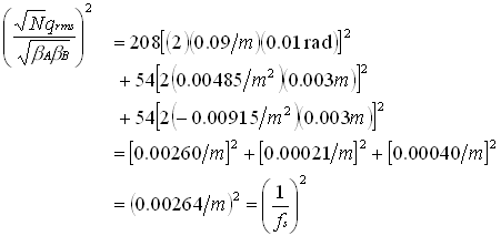 (20)
(20)
So the contribution from the quads dominates. Take the factor ![]() to be about the same at the
skew quad as at a normal quad or sextupole. Then the required skew quad inverse focal
length is 0.0026/m. This is about 1/35 of a normal quad. This only looks at the
magnitude of the coupling and ignores the phase of the coupling wave.
to be about the same at the
skew quad as at a normal quad or sextupole. Then the required skew quad inverse focal
length is 0.0026/m. This is about 1/35 of a normal quad. This only looks at the
magnitude of the coupling and ignores the phase of the coupling wave.
From equations (17) and (20), the uncorrected minimum tune split will be
 (21)
(21)
where typical b have been used. If we only require
that we can make the tunes equal (global decoupling), then by equation (17) we only need
control over ![]() +,the
components of
+,the
components of ![]() that propagate as
the difference of the normal mode phase advances. So in this case only 2 nondegenerate
skew quads will be needed. For the
that propagate as
the difference of the normal mode phase advances. So in this case only 2 nondegenerate
skew quads will be needed. For the ![]() +, nondegenerate means that (fA,12
- fB,12)¹0 is
sufficient, (fA,12 - fB,12)=(0.25)2p would be optimal, resulting in the skew quads producing orthogonal
effects at the coupling resonance
+, nondegenerate means that (fA,12
- fB,12)¹0 is
sufficient, (fA,12 - fB,12)=(0.25)2p would be optimal, resulting in the skew quads producing orthogonal
effects at the coupling resonance
At present the two transverse tunes of the main injector are both about 22.42 and the phases of the normal modes advance together. So the quantity (fA - fB) varies by about (0.1)2p, but the locations where we would like to place the skew quads are already occupied by other magnets. (These locations are roughly at the boints whtere the bA»bB as the mode whose b goes through a minimum between these pints has a fairly large phase advance, wherease the mode whose b goes through a maximum between these poi8nts has a fairly small phase advance.) Fortunately there are several empty cells where there is still a veriation of about (0.1)2p) in (fA - fB), and there are no other magnets in the way. While not optimal, this is sufficient; but since the skew quads are not orthogonal, they will generally have to be run stronger.
Prompted by reasons other than coupling, there is a movement afoot to separate the integer tunes by 1 unit. If this is done, then at locations separated by about 1/4 of the ring, the difference in (fA - fB) will be our ideal (0.25)2p. So considering only the correction of the global coupling, separating the integer tunes by one or more units is desirable, but not absolutely necessary.
The local coupling is parametrized by the ![]() . Recall equations (6) and (9) which give the
. Recall equations (6) and (9) which give the ![]() in terms of the
in terms of the ![]() and the
and the ![]() in terms of the
in terms of the ![]() ±**
±**
 (22)
(22)
With the fractional tunes so close the ![]() are dominated by the
are dominated by the ![]() +
terms. However, equation (17) shows that global decoupling makes
+
terms. However, equation (17) shows that global decoupling makes ![]() +=0 on the
coupling resonance. Since the design tundes are near the coupling resonance, the
+=0 on the
coupling resonance. Since the design tundes are near the coupling resonance, the ![]() + will still be small at
the design tunes. The
+ will still be small at
the design tunes. The ![]() -
term, although not resonant at nA˜nB, may still be appreciable. Use equations (14) and
(20) to extimate (
-
term, although not resonant at nA˜nB, may still be appreciable. Use equations (14) and
(20) to extimate (![]() -)rms
where
-)rms
where
 (23)
(23)
g is very nearly 1 as long as Tr2(A-B)
>> 4det![]() , that is as
long as the machine is not on the coupling resonance. Although quite small, an unusually
bad set of errors could give 2 or 3 times this amount and
, that is as
long as the machine is not on the coupling resonance. Although quite small, an unusually
bad set of errors could give 2 or 3 times this amount and ![]() - of about 0.1 could begin
to be a problem. So we would like to control these as well and that requires two more
nondegenerate skew quads. These components propogate as the sum of the normal mode phase
advances, and so advance by about 45(2p) radians around the
ring. Consequently it is easy to find optimal locations for these additional skew quads.
With 4 skew quads in the ring, we could locally decouple (make the matrix
- of about 0.1 could begin
to be a problem. So we would like to control these as well and that requires two more
nondegenerate skew quads. These components propogate as the sum of the normal mode phase
advances, and so advance by about 45(2p) radians around the
ring. Consequently it is easy to find optimal locations for these additional skew quads.
With 4 skew quads in the ring, we could locally decouple (make the matrix ![]() =0) the machine at one point. In
effect, we could close the coupling bump.
=0) the machine at one point. In
effect, we could close the coupling bump.
We have looked at the coupling that will be produced by roll angles of normal quads and vertical displacements within sextupoles and seen that most of the coupling is from the roll angles. Without any skew quads to correct this coupling, we expect a minimum tune split of about 0.010. In order to bring the tunes together (globally decouple the machine), we will need two orthogonal skew quads with inverse focal lengths of about 0.0026/m, about 1/35 the strenght of a normal quad. The coupling components that contribute to the global coupling propagate as the difference of the normal mode phase advances. For tunes of 22.42 and 22.43, the normal mode phases advance together, so there is not much variation in the difference in the normal mode phase advances. Consequently there are no locations for the skew quads where they will be Orthogonal (difference in normal mode phase advances of (0.25)2p). About the best that can be done is a difference in normal mode phase advance of about (0.1)2p, so we would be wise to double their maximum strenths. Also since the above value is based on rms errors, we would not be surprised if the actual errors were 3 to 5 times larger. So we would like two skew quads with maximum strengths of about 2×4×0.0026/m=0.021/m, or about 1/4 the strength of a normal quad. If the integer tunes are seperates by 1 or more units, optimal locations will exist and about half this mazimum strength will suffice.
Once the machine is globally decoupled, there will still be local coupling of ![]() ˜.036. Most of this will be the
coupling component that propagates like the sum of the normal mode phase advances. So in
order to adjust this independently of the global coupling, we would like two more skew
quads. Since in going around the ring, the sum of the normal mode phase advances goes
through about 45(2p) radians, there is no problem finding
orthogonal locations for these skew quads and maximum strengths of about 0.015/m,
or about 1/8 the strenght of a normal quad, should suffice.
˜.036. Most of this will be the
coupling component that propagates like the sum of the normal mode phase advances. So in
order to adjust this independently of the global coupling, we would like two more skew
quads. Since in going around the ring, the sum of the normal mode phase advances goes
through about 45(2p) radians, there is no problem finding
orthogonal locations for these skew quads and maximum strengths of about 0.015/m,
or about 1/8 the strenght of a normal quad, should suffice.
*Tr2(A-B) has the same value at all points on the ring.
Generally both Tr2(M-N) and det![]() vary from point to point in the ring.
Specifically they are constant between couplers and change at the couplers. However at the
coupling resonance, the changes at the couplers goes to zero, det
vary from point to point in the ring.
Specifically they are constant between couplers and change at the couplers. However at the
coupling resonance, the changes at the couplers goes to zero, det![]() has the same value at all points in
the ring and Tr(M-N) is zero everywhere.
has the same value at all points in
the ring and Tr(M-N) is zero everywhere.
** Despite appearances in equation (22), the ![]() remain finite at nA = nB. This is because near the coupling resonance the
difference i ntundes is related to the det
remain finite at nA = nB. This is because near the coupling resonance the
difference i ntundes is related to the det![]() . See equation (7).
. See equation (7).