MI-0250
Stripline Detectors for Fermilab Main Injector
Jim
Crisp[1],
Konstantin Gubrienko[2],
and Vladimir Seleznev[2]
December 7, 1998
Stripline Detectors for Fermilab Main Injector
Jim
Crisp[3],
Konstantin Gubrienko[4], and
Vladimir Seleznev2
Introduction
The Institute for High Energy
Physics designed and built four stripline beam detectors for use at
Fermilab. The detectors will be installed
for general purpose use, two in the Main Injector and two in the Recycler. A round geometry with two stripline plates
was chosen to allow installation as either horizontal or vertical position
detectors. Electrical feedthroughs at
both ends of the 1.4 meter long striplines allow measurement of both proton and
antiproton signals. The 1 gigahertz
bandwidth and 9.3 nsec doublet separation allow measurement of high frequency
structure within the beam bunches.
Design features
The striplines are mounted in a
150 mm ID stainless tube. Torlon 4203
(made by Amoco Chemicals Corp.) was selected to make the insulators which hold
the striplines in position. Torlon has
a tensile strength of 22000 psi, is resistant to radiation damage, is easily
machineable, can be baked to 260°C, and has good vacuum properties.
The 60 degree wide plates
intercept and carry about 1/6 of the beam image current. The peak amplitude on the 50Ω plates
will be about 10 volts for 6e10 protons in a 3 nsec sigma gaussian bunch. A plate length of 1.4 meters (l/4 wavelength
at the rf frequency of 53 MHz) is used to maximize the doublet separation. In the time domain, this allows observation
of the bunch shape and changes in position along it's length. In the frequency domain, zero's in transmission
occur when the plate is a multiple of 1/2 wavelengths long. This occurs at even harmonics of the rf
frequency.
Figure
1. Cross section of stripline detector.
Type N vacuum feedthroughs are
used at each end to access the signals.
To allow easy replacement, the feedthroughs are welded into vacuum
flanges and the center pin makes electrical contact by depressing stainless
tabs on the stripline.
The detectors are placed in
regions having 6 inch round vacuum tube.
Both the Main Injector and Recycler use elliptical shaped vacuum tube
through most of their circumference. A
smooth transition between the two shapes is used to minimize beam
impedance. The microwave cut off
frequency has been measured to be 1.2 GHz in the striplines and 1.5 GHz in the
elliptical pipe.
Ideal Stripline response
Beam traveling along a vacuum
tube induces image charge of equal but opposite sign on the conducting
walls. About 1/6th of this charge will
be induced onto the plate at the upstream end and removed at the downstream
end. The frequency response can be
estimated by summing the voltage produced from these two opposing current
sources taking into account their time difference. The voltage at both ends as a function of frequency is estimated
below for a 60° wide plate, length (l), impedance (Zo), and beam velocity (c).
Ideal
stripline frequency response
All charge induced on the
upstream end will be removed at the downstream end as the beam exits the
detector. No signal is produced at the
downstream end of an ideal stripline provided the charge on the plate travels
at the same velocity as the beam and exactly matches the image charge removed
as the beam passes the downstream end.
This also requires a constant plate impedance and perfect match to the
signal cables.
The two striplines within a
detector couple to each other making their impedance depend on the balance of
charge, or beam position. For the
geometry used, the plate impedance is reduced by 3Ω when driven
differentially. This calculation was
verified using time domain reflectometry.
Thus, directionality depends on beam position.
Wire Measurements
The cutoff frequency for the
TE11 mode inside the stripline is about 1.2 GHz making the response irregular
and unusable above this frequency.
Below cut off, there is excellent agreement with an ideal
stripline. The measurements shown below
were made by driving a wire placed along the center of the detector. Resistive dividers were used to minimize
reflections on the wire by matching the impedance to 50Ω at each
end. Transmission through the wire was
flat to ±1 db.
Figure
2. Measured, calculated, and ideal
stripline response at the upstream end.
The calculation used 53Ω lines terminated with 50Ω in
parallel with 4pf.
Figure
3. Measured and calculated stripline
response at the downstream end. The
calculation was done with and without 4pf at the ends.
The model uses two current
sources with the correct time difference and polarity driving both ends of a
53Ω transmission line. Good
agreement with measurement was obtained by terminating the lines with 50Ω
in parallel with 4pf capacitors. The
measured amplitude indicates about 1/4 of the beam current is induced on to the
plates.
The excess capacitance at the
ends is caused by the geometry used to hold the striplines in position. Mismatch from this capacitance causes
reflections which reduce the directionality of the detectors. Because protons and antiprotons are never in
the Main Injector or Recycler at the same time, directionality is not important
for this application.
The log of the ratio of the
signals on the two striplines is proportional to position. The sensitivity is 2mm/db through 75% of
the 110 mm aperture as shown below.

Figure
4. A/B scaled by 2mm/db for wire
positions from 0 to 50 mm in 5 mm steps versus frequency and at 1, 3, 5, 7, and
9 times 53 MHz versus wire position.
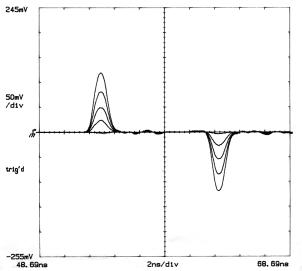
The time domain response was
measured with a gaussian shaped pulse having a sigma width of 0.5 nsec, the
shortest length we could easily generate.
The pulse traveled along a wire placed at the center of the detector. The Fourier transform of a gaussian pulse is
itself a gaussian having a sigma width of 320 MHz. The frequency components of such a pulse fall easily within the
bandwidth of the detector as evidenced by the excellent agreement between
measurement and the model shown below.

Figure
5. Measured and calculated response to
gaussian pulse with 0.5 nsec sigma width.
Figure
6. Measured and calculated response to
gaussian pulse with 0.5 nsec sigma width at the downstream end.
Beam position can be estimated
with the ratio of the difference to the sum of the two stripline signals. Excellent position sensitivity with a well
behaved time structure was measured by changing the wire position and taking
the difference between the two striplines, shown below.
Figure
7. A-B for 0, 10, 20, 30, and 40 mm
wire position.
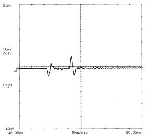
Beam Measurement
On October 10th, beam was
successfully circulated around the new Fermilab Main Injector. Intensities were limited to avoid
unnecessary contamination, but 5e10 protons in 84 bunches were routinely
circulated without rf for 25 seconds when they were intentionally aborted. The figure below was taken on the first turn
while beam was still longitudinally bunched.
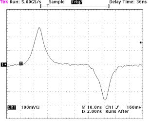
Figure
8. A+B produced with circulating beam
in the Fermilab Main Injector.
Conclusion.
The only significant
improvements to the existing design would be to reduce the capacitance at the
ends of the plates and perhaps adjust the plate position slightly to make them
50Ω.
Fermilab is grateful for the
excellent detectors designed and built by IHEP. Their response is nearly ideal and will provide excellent
measurements for years to come.